<?xml version="1.0" encoding="utf-8"?><feed xmlns="http://www.w3.org/2005/Atom" ><generator uri="https://jekyllrb.com/" version="4.4.1">Jekyll</generator><link href="https://finance.abdulmalik.de/feed.xml" rel="self" type="application/atom+xml" /><link href="https://finance.abdulmalik.de/" rel="alternate" type="text/html" /><updated>2026-06-20T11:57:20+02:00</updated><id>https://finance.abdulmalik.de/feed.xml</id><title type="html">Abdul Malik | Finance &amp;amp; Technology</title><subtitle>Writing about quantitative finance, capital markets, machine learning, and financial technology.</subtitle><author><name>Abdul Malik</name><email>abdul.malik.work@gmail.com</email></author><entry><title type="html">What I Learned After Running an LLM Portfolio for Five Years</title><link href="https://finance.abdulmalik.de/2026/06/10/what-i-learned-running-an-llm-portfolio/" rel="alternate" type="text/html" title="What I Learned After Running an LLM Portfolio for Five Years" /><published>2026-06-10T00:00:00+02:00</published><updated>2026-06-10T00:00:00+02:00</updated><id>https://finance.abdulmalik.de/2026/06/10/what-i-learned-running-an-llm-portfolio</id><content type="html" xml:base="https://finance.abdulmalik.de/2026/06/10/what-i-learned-running-an-llm-portfolio/"><![CDATA[<p>When I started this research, I expected the AI portfolio to win.</p>

<p>A large language model can process earnings calls, Federal Reserve communications, market indicators, and macroeconomic data all at once. That is roughly what experienced investors do when they sit down to make allocation decisions. The bet was that doing it at scale, across thousands of documents, would improve the result.</p>

<p>It did not.</p>

<p>Over the five-year out-of-sample period, the LLM-enhanced portfolio generated a Sharpe Ratio of 0.767. The strongest quantitative benchmark came in at 0.856. Looking at those numbers on their own, the conclusion seems simple: the AI did not work.</p>

<p>But the numbers were hiding something.</p>

<hr />

<h2 id="the-results">The Results</h2>

<p>Here is how the main strategies compared across the full evaluation period:</p>

<table>
  <thead>
    <tr>
      <th>Strategy</th>
      <th>Sharpe Ratio</th>
    </tr>
  </thead>
  <tbody>
    <tr>
      <td>Minimum Variance</td>
      <td>0.879</td>
    </tr>
    <tr>
      <td>Signal-Enhanced Minimum Variance</td>
      <td>0.856</td>
    </tr>
    <tr>
      <td>LLM-Enhanced Portfolio</td>
      <td>0.767</td>
    </tr>
  </tbody>
</table>

<p>The LLM underperformed both quantitative benchmarks, including the Signal-Enhanced portfolio that already incorporated momentum signals, volatility regime adjustments, and yield curve data. On a pure risk-adjusted basis, there was no case for the AI approach.</p>

<p>One number did not fit neatly into that picture. The LLM-enhanced portfolio generated a statistically significant Fama-French alpha, meaning the model was capturing information that standard risk factors do not explain. It was not producing random noise. Something real was being picked up; it just was not making its way into better returns. Figuring out why that gap existed became the most instructive part of the whole project.</p>

<hr />

<h2 id="why-the-llm-lost">Why the LLM Lost</h2>

<h3 id="the-correlation-problem">The Correlation Problem</h3>

<p>The portfolio universe was ten U.S. equity ETFs, and they are not independent assets.</p>

<p>Technology, growth, and large-cap equities move together across most market environments. Energy and financials have their own dynamics, but the universe was still heavily correlated on average. When assets move together like that, rotating between them does not produce much in the way of active returns. There was a structural ceiling on what any tactical allocation model could achieve here, and the LLM was up against it from the start.</p>

<h3 id="the-noise-problem">The Noise Problem</h3>

<p>To reduce randomness in the outputs, I ran Llama 3.1 8B five times each month and averaged the results. That helped, but language models are stochastic: the same inputs do not always produce the same outputs. Each monthly run could return meaningfully different portfolio weights. Averaged across five runs the signal-to-noise ratio improved, but it was never clean. Over five years of monthly decisions, that noise accumulates and it drags on performance.</p>

<hr />

<h2 id="the-ridge-regression-test">The Ridge Regression Test</h2>

<p>At some point I started asking a question I probably should have asked earlier: was the value coming from the LLM, or from the features it was given?</p>

<p>The model was working with earnings sentiment features, Fed sentiment features, momentum signals, volatility data, and yield curve information. Those inputs might carry predictive power on their own, regardless of how they are processed. To check, I trained a Ridge Regression model on exactly the same features.</p>

<table>
  <thead>
    <tr>
      <th>Strategy</th>
      <th>Sharpe Ratio</th>
    </tr>
  </thead>
  <tbody>
    <tr>
      <td>Ridge Regression</td>
      <td>0.870</td>
    </tr>
    <tr>
      <td>LLM-Enhanced Portfolio</td>
      <td>0.767</td>
    </tr>
  </tbody>
</table>

<p>The simple regularised model beat the LLM by a substantial margin.</p>

<p>That result reframed the picture. The features contained genuine predictive information. The LLM was not using them better than a well-tuned linear model. If anything, it was using them worse. The value was in the data, not in the reasoning layer on top.</p>

<hr />

<h2 id="the-discovery-that-changed-my-conclusion">The Discovery That Changed My Conclusion</h2>

<p>The overall Sharpe numbers pointed one way: quantitative models win, close the notebook.</p>

<p>Breaking the results down by time period told a different story:</p>

<table>
  <thead>
    <tr>
      <th>Period</th>
      <th>LLM Sharpe Ratio</th>
    </tr>
  </thead>
  <tbody>
    <tr>
      <td>2021 to 2022</td>
      <td>0.603</td>
    </tr>
    <tr>
      <td>2023 to 2025</td>
      <td>0.968</td>
    </tr>
  </tbody>
</table>

<p>Same model, same architecture, same features, but completely different performance depending on what the market was doing. Averaged across five years the LLM looked mediocre. Split into two periods it looked like two different models. The aggregate number was not wrong, it was just not asking the right question.</p>

<hr />

<h2 id="when-the-ai-actually-worked">When the AI Actually Worked</h2>

<p>November 2023 is the clearest example of the model doing what it was built for.</p>

<p>The Fed had been hiking aggressively throughout 2022 and into 2023. By late 2023, inflation was coming down and the language coming out of the FOMC was shifting. The pivot from tightening to pausing was becoming visible in the text before it showed up clearly in the data.</p>

<p>The model saw it. Earnings calls across technology and consumer sectors were turning more optimistic. Fed communications were softening on inflation. Importantly, the model’s five runs that month came back with similar answers, which is what a high confidence score reflects in this system. It rotated toward growth with some conviction.</p>

<p>That call worked. Growth equities ran through the first half of 2024, and the portfolio was already there.</p>

<hr />

<h2 id="when-the-ai-failed">When the AI Failed</h2>

<p>March 2025 looked completely different.</p>

<p>Tariff announcements were creating sharp uncertainty. Earnings calls were contradictory: companies were reporting decent recent results while simultaneously pulling forward guidance and flagging supply chain risk. The macro picture was moving faster than the corporate fundamentals. Earnings sentiment came in cautiously positive, Fed communications were hawkish, volatility was elevated, and yield curve signals were ambiguous. The signals pointed everywhere at once.</p>

<p>The model had no way to make sense of that, but it did not say so. Across five runs, it produced high confidence scores. Reading through the outputs, I found something specific: the model was referencing an inverted yield curve in its reasoning when the yield curve was not actually inverted. It had filled in context that was not there, and it had done it with apparent certainty.</p>

<p>That is a different problem from getting the allocation wrong. A bad call can come from bad luck or an unusual environment. Generating false context while appearing certain is a structural issue with how the confidence mechanism was working.</p>

<hr />

<h2 id="the-real-contribution">The Real Contribution</h2>

<p>The key lesson was not the headline result. It was understanding when the model should and should not be trusted.</p>

<p>The confidence mechanism counted how many signals were firing above a threshold. More signals meant higher confidence. That works when markets are coherent. It breaks down when markets are full of contradictory information, because activity and agreement are not the same thing.</p>

<p>November 2023 worked because everything pointed in the same direction. Earnings sentiment, Fed tone, and macro signals were all telling a consistent story, and the five model runs agreed with each other. Confidence was high because agreement was high.</p>

<p>In March 2025, signals were active and contradictory. The confidence score was high because a lot was happening, not because any clear picture was forming. The mechanism measured volume when it should have been measuring coherence. A better system would distinguish between those two states: not just how many signals are firing, but whether they are saying the same thing.</p>

<hr />

<h2 id="final-thoughts">Final Thoughts</h2>

<p>The thesis did not establish that LLMs outperform quantitative models. The numbers are clear on that.</p>

<p>What it did show is that qualitative information is not irrelevant to portfolio decisions. The Fama-French alpha was real. The November 2023 call was not an accident. The signal was there; the architecture was not yet good enough to use it reliably under all conditions.</p>

<p>Small open-source models run locally are probably better understood as feature processors right now than as autonomous portfolio decision makers. They can translate text into signals. Synthesising those signals under ambiguous market conditions, without hallucinating context or overclaiming certainty, is still a hard problem.</p>

<p>The regime results leave room for optimism. More capable models, a confidence framework built around signal coherence rather than signal volume, and better access to real-time information could change what is achievable here. That is worth building toward.</p>

<p>Language carries information that moves markets. Extracting it reliably, without the noise eating the signal, is the part that still needs work.</p>]]></content><author><name>Abdul Malik</name><email>abdul.malik.work@gmail.com</email></author><category term="Articles" /><category term="Portfolio Management" /><category term="AI" /><category term="LLMs" /><category term="Quantitative Finance" /><category term="FinTech" /><category term="Frankfurt School" /><summary type="html"><![CDATA[When I started this research, I expected the AI portfolio to win.]]></summary><media:thumbnail xmlns:media="http://search.yahoo.com/mrss/" url="https://finance.abdulmalik.de/assets/images/LLM-Portfolio_2.png" /><media:content medium="image" url="https://finance.abdulmalik.de/assets/images/LLM-Portfolio_2.png" xmlns:media="http://search.yahoo.com/mrss/" /></entry><entry><title type="html">Building an AI Portfolio Manager: Can LLMs Beat Quant Investing?</title><link href="https://finance.abdulmalik.de/2026/06/04/building-an-ai-portfolio-manager/" rel="alternate" type="text/html" title="Building an AI Portfolio Manager: Can LLMs Beat Quant Investing?" /><published>2026-06-04T00:00:00+02:00</published><updated>2026-06-04T00:00:00+02:00</updated><id>https://finance.abdulmalik.de/2026/06/04/building-an-ai-portfolio-manager</id><content type="html" xml:base="https://finance.abdulmalik.de/2026/06/04/building-an-ai-portfolio-manager/"><![CDATA[<p>Numbers run portfolio management. That sounds obvious, but it shapes everything: how risk is measured, how capital is allocated, which decisions get made and which get ignored.</p>

<p>Investors build models around returns, volatility, correlations, yield spreads, valuation metrics, and factor exposures. From Markowitz to modern factor investing, the toolkit has stayed largely quantitative.</p>

<p>And yet every quarter, thousands of companies tell investors exactly how they see the future.</p>

<p>Executives discuss demand trends, competitive pressures, supply chain issues, hiring plans, capital expenditure programs, and growth expectations during earnings calls. The Federal Reserve communicates its read on inflation, growth, labour markets, and rate policy through statements, minutes, and press conferences. Professional investors spend enormous amounts of time working through all of it.</p>

<p>So the question I kept coming back to was whether an AI could do the same: could a Large Language Model improve portfolio performance by combining qualitative signals from earnings calls and Fed communications with traditional quantitative data?</p>

<p>That question became the foundation of my master’s thesis in Portfolio Management at Frankfurt School of Finance &amp; Management. Twelve thousand earnings call transcripts, hundreds of Federal Reserve documents, and thousands of AI-generated portfolio decisions later, I had an answer I did not expect.</p>

<hr />

<h2 id="the-traditional-approach-to-portfolio-construction">The Traditional Approach to Portfolio Construction</h2>

<p>Most portfolio models are fundamentally backward-looking.</p>

<p>They use historical returns to estimate risk and expected performance, identifying patterns such as momentum, volatility regimes, or factor exposures and allocating capital accordingly. These approaches work because markets often exhibit persistent behaviour. Assets that have performed well recently may continue to do so. Volatility regimes shape investor risk appetite. Certain sectors tend to outperform in specific economic environments.</p>

<p>What traditional models routinely ignore is language.</p>

<p>A technology company reports earnings: revenue beats expectations, margins improve, management raises guidance. Separately, the Federal Reserve signals that inflation risks are fading and rate cuts are becoming more likely. Both events carry information that may move prices. But converting thousands of pages of financial text into investable signals has historically been hard to do well, and most quantitative frameworks do not try.</p>

<p>That started to change with the development of large language models.</p>

<hr />

<h2 id="the-rise-of-financial-language-models">The Rise of Financial Language Models</h2>

<p>Natural language processing looked very different ten years ago.</p>

<p>Early approaches relied on dictionaries that mapped words to positive or negative scores. These worked poorly in finance, where “liability” or “debt” sound alarming in everyday language but carry neutral or routine meanings in a corporate filing.</p>

<p>Transformer models changed things. BERT, FinBERT, GPT, Llama, and Mistral can process language in context rather than scoring words in isolation. FinBERT, trained specifically on financial text, became one of the more widely used tools for financial sentiment analysis.</p>

<p>Large language models added something beyond that: the ability to hold multiple signals in mind at once. An LLM can take in positive earnings sentiment alongside a deteriorating macroeconomic outlook, an inverted yield curve, and rising volatility, and try to arrive at a coherent view. Whether doing that actually improves portfolio decisions was a question that had not really been tested at the portfolio level.</p>

<hr />

<h2 id="designing-the-experiment">Designing the Experiment</h2>

<p>Rather than studying individual stock predictions, I wanted to test something more practical: whether an LLM could improve an entire portfolio allocation process.</p>

<p>I built a universe of ten major U.S. equity ETFs covering different sectors, styles, and market-cap segments: broad S&amp;P 500 exposure, technology, financials, healthcare, energy, growth, value, and mid-to-small cap equities. The portfolio was rebalanced monthly, and each month followed the same process.</p>

<h3 id="step-1-build-a-quantitative-baseline">Step 1: Build a Quantitative Baseline</h3>

<p>A minimum-variance portfolio was constructed using an exponentially weighted covariance matrix, creating a quantitative benchmark based purely on market data.</p>

<h3 id="step-2-extract-information-from-text">Step 2: Extract Information from Text</h3>

<p>I collected 12,364 earnings call transcripts and 347 Federal Reserve documents, including FOMC statements, meeting minutes, and press conference transcripts. All were processed through FinBERT.</p>

<p>The resulting sentiment features captured overall earnings tone, forward guidance sentiment, management confidence, Federal Reserve communication style, inflation concerns, economic outlook signals, and labour market assessments.</p>

<h3 id="step-3-let-the-llm-make-portfolio-decisions">Step 3: Let the LLM Make Portfolio Decisions</h3>

<p>Llama 3.1 8B was deployed locally using Ollama. Each month, the model received the baseline portfolio weights alongside momentum signals, volatility data, yield curve information, macroeconomic indicators, and the earnings and Fed sentiment features, then proposed revised weights.</p>

<p>To reduce randomness, I ran the model five times each month and averaged the results. Across the full study, that produced 960 independent LLM portfolio decisions.</p>

<hr />

<h2 id="the-benchmark-problem">The Benchmark Problem</h2>

<p>A lot of AI investment research compares against weak baselines. A model beats an equal-weight portfolio and claims it works. That is not a meaningful test.</p>

<p>The real question is whether an LLM can outperform a strategy that already incorporates well-known predictive signals. So I compared the LLM portfolio against five alternatives: Minimum Variance, Risk Parity, Equal Weight, Value Tilt, and Signal-Enhanced Minimum Variance.</p>

<p>The Signal-Enhanced portfolio was the one that mattered most. It already included momentum signals, volatility regime adjustments, and yield curve information, representing what a strong quantitative model could do with market data alone. The LLM needed to beat that to show that reading earnings calls and Fed minutes was actually adding something beyond what the numbers already said.</p>

<hr />

<h2 id="what-i-expected">What I Expected</h2>

<p>I thought the LLM would find relationships that traditional quantitative models missed: strong earnings optimism combined with a dovish Fed shift, sector-specific divergence in management confidence, narratives that were changing before the data caught up. These are exactly the kinds of signals that experienced analysts look for, and they are difficult to capture with linear models.</p>

<p>The reasoning seemed sound. Professional investors spend significant time interpreting these sources. A model that could process them at scale should, in theory, pick up something useful.</p>

<p>It was more complicated than that.</p>

<p>After processing over twelve thousand earnings calls and hundreds of Federal Reserve documents, the results pushed back on a lot of what I had assumed going in. What worked, what failed, and why it failed were not the story I had written in my head before the data came in.</p>

<p>That is what the next article covers.</p>]]></content><author><name>Abdul Malik</name><email>abdul.malik.work@gmail.com</email></author><category term="Articles" /><category term="Portfolio Management" /><category term="AI" /><category term="LLMs" /><category term="Quantitative Finance" /><category term="FinTech" /><category term="Frankfurt School" /><summary type="html"><![CDATA[Numbers run portfolio management. That sounds obvious, but it shapes everything: how risk is measured, how capital is allocated, which decisions get made and which get ignored.]]></summary><media:thumbnail xmlns:media="http://search.yahoo.com/mrss/" url="https://finance.abdulmalik.de/assets/images/LLM-Portfolio_1.png" /><media:content medium="image" url="https://finance.abdulmalik.de/assets/images/LLM-Portfolio_1.png" xmlns:media="http://search.yahoo.com/mrss/" /></entry><entry><title type="html">Europe’s Balancing Act with the Digital Euro</title><link href="https://finance.abdulmalik.de/2026/03/20/digital-euro-europes-balancing-act/" rel="alternate" type="text/html" title="Europe’s Balancing Act with the Digital Euro" /><published>2026-03-20T00:00:00+01:00</published><updated>2026-03-20T00:00:00+01:00</updated><id>https://finance.abdulmalik.de/2026/03/20/digital-euro-europes-balancing-act</id><content type="html" xml:base="https://finance.abdulmalik.de/2026/03/20/digital-euro-europes-balancing-act/"><![CDATA[<p>Central banks around the world are building digital currencies. But they are not all solving the same problem.</p>

<p>China’s digital yuan is partly about scale and state-backed payment infrastructure. The Bahamas’ Sand Dollar was built around access and inclusion. Other CBDC projects focus on payments modernisation or reducing dependence on cash.</p>

<p>The Digital Euro is different. It is Europe’s attempt to update public money for a digital economy without blowing up the role of private banks.</p>

<p>That tension matters more than the technology behind it.</p>

<hr />

<h2 id="what-europe-is-actually-building">What Europe Is Actually Building</h2>

<p>The ECB’s own framing is careful. A digital euro would be a digital form of central bank money for everyday payments, available across the euro area, designed to complement cash rather than replace it. The current model does not imagine citizens opening accounts directly with the ECB. Distribution would run through supervised intermediaries, banks and payment service providers, which would remain the customer-facing layer.</p>

<p>There is also a sovereignty argument running through this. Cash use is falling across the euro area, and the payment rails that have filled the gap are mostly foreign: American card networks, US-headquartered tech platforms. The ECB has been candid that preserving a European form of public money, one not controlled by a private company or a foreign government, is part of what this project is about.</p>

<p>The ECB completed its investigation phase in 2023 and has since been working through the technical design, legislation, and coordination with commercial banks. No final decision to issue has been made yet.</p>

<hr />

<h2 id="why-banks-sit-at-the-centre-of-the-debate">Why Banks Sit at the Centre of the Debate</h2>

<p>For users, a Digital Euro payment could feel almost uneventful. One scenario the ECB has designed for: you pay at a market stall with no internet connection, the transaction settles offline between devices, and the merchant’s balance updates when connectivity returns. That is something cards and apps currently cannot do, and it is one of the more concrete use cases being built around.</p>

<p>For banks, none of this is uneventful.</p>

<p>Retail deposits are one of the foundations of commercial banking. They help fund lending, support liquidity, and anchor the customer relationship. A retail CBDC introduces a new form of money that could compete with those deposits, particularly if consumers see central bank money as safer in times of stress.</p>

<p>That is why the Digital Euro is being designed with guardrails. The ECB has discussed holding limits of around 3,000 euros per person, keeping it useful as a payment tool while making it unattractive as a savings vehicle. Europe wants people to use the Digital Euro for paying, not for moving large sums out of bank deposits.</p>

<p>Banks and payment firms would still handle onboarding, wallets, customer support, fraud monitoring, compliance, and integration into existing apps. The ECB issues the money; the private sector shapes the experience. How intermediaries get compensated for that work, given the Digital Euro pays no interest, is a question the ECB has not fully resolved publicly.</p>

<hr />

<h2 id="how-it-compares-with-other-models">How It Compares With Other Models</h2>

<h3 id="chinas-e-cny">China’s e-CNY</h3>

<p>China’s digital yuan is further along in pilot deployment. It uses authorised operators to distribute it and offers what official descriptions call “managed anonymity,” meaning transaction data can be accessed by the state under certain conditions but is not routinely visible to operators. That makes it a serious retail payments instrument, but one built around very different assumptions about government access than Europe would accept.</p>

<h3 id="the-bahamas-sand-dollar">The Bahamas’ Sand Dollar</h3>

<p>The Sand Dollar addressed financial inclusion across a dispersed island geography where traditional banking was uneven. Europe does not face that problem at scale. Its challenge is not expanding access to money, but preserving the role of public money in a market already crowded by banks, cards, large payment platforms, and private stablecoins now regulated under MiCA.</p>

<hr />

<h2 id="why-privacy-matters-so-much-in-europe">Why Privacy Matters So Much in Europe</h2>

<p>The Digital Euro will not be judged by architecture diagrams. It will be judged by a simpler question: <em>who can see my payments?</em></p>

<p>The ECB says it would not identify people from their payment data and has designed offline functionality partly to offer privacy levels closer to cash, where only payer and payee know a transaction happened. But the project must also operate within EU anti-money laundering rules, which require some transaction visibility. Those two things are in direct tension, and the legislation working through Brussels has not settled it cleanly.</p>

<p>That unresolved tension is what makes the Digital Euro genuinely interesting to watch.</p>

<p>Not because it is “digital,” since most money already is, but because Europe is trying to redesign money without breaking the banking model underneath it.</p>

<p>If it succeeds, the result may feel almost uneventful to the average user. That would be a job well done.</p>]]></content><author><name>Abdul Malik</name><email>abdul.malik.work@gmail.com</email></author><category term="Articles" /><category term="Digital Euro" /><category term="CBDC" /><category term="ECB" /><category term="Central Banking" /><category term="Monetary Policy" /><category term="FinTech" /><summary type="html"><![CDATA[Central banks around the world are building digital currencies. But they are not all solving the same problem.]]></summary><media:thumbnail xmlns:media="http://search.yahoo.com/mrss/" url="https://finance.abdulmalik.de/assets/images/Digital_Euro.png" /><media:content medium="image" url="https://finance.abdulmalik.de/assets/images/Digital_Euro.png" xmlns:media="http://search.yahoo.com/mrss/" /></entry><entry><title type="html">Reading the Tape on Twitter</title><link href="https://finance.abdulmalik.de/2026/03/13/financial-tweet-sentiment/" rel="alternate" type="text/html" title="Reading the Tape on Twitter" /><published>2026-03-13T00:00:00+01:00</published><updated>2026-03-13T00:00:00+01:00</updated><id>https://finance.abdulmalik.de/2026/03/13/financial-tweet-sentiment</id><content type="html" xml:base="https://finance.abdulmalik.de/2026/03/13/financial-tweet-sentiment/"><![CDATA[<p>Financial markets move on information, and increasingly, that information flows through social media before it reaches anywhere else. A tweet from an analyst, a headline reposted by a trader, a single word like “downgrade” are all signals that can move prices. The question this project explores is simple: <strong>Can a machine be trained to reliably tell a bullish post from a bearish one?</strong></p>

<hr />

<h2 id="the-data">The Data</h2>

<p>The dataset contains <strong>9,543 financial tweets</strong>, each labelled as Bearish, Bullish, or Neutral. Since the goal is binary classification, Neutral tweets were removed, leaving <strong>3,365 tweets</strong> split roughly 57% Bullish and 43% Bearish.</p>

<p><img src="/assets/images/classdistribution_twitter.png" alt="Class distribution and tweet length by sentiment" /></p>

<p>
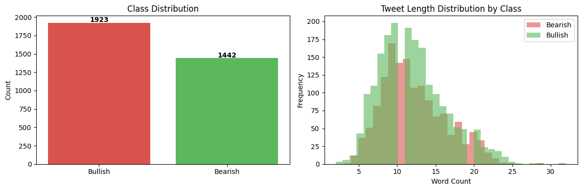
The class imbalance is modest but worth noting. There are more Bullish tweets than Bearish ones in the data, which subtly influences how models behave. Interestingly, Bearish and Bullish tweets are nearly identical in length, so tweet length alone tells us nothing useful about sentiment.</p>

<hr />

<h2 id="turning-words-into-numbers">Turning Words Into Numbers</h2>

<p>Computers cannot deterministically make sense of text. They read numbers. The core challenge in any text classification problem is finding the right way to convert language into something a model can learn from.</p>

<p>Two approaches were used here:</p>

<p><strong>TF-IDF (Term Frequency–Inverse Document Frequency)</strong> treats each word (and two-word phrase) as a feature and scores it by how often it appears in a tweet relative to how common it is across all tweets. A word like “downgrade” that appears frequently in Bearish tweets but rarely overall gets a high score. A word like “the” that appears everywhere gets a low score.</p>

<p>Before applying TF-IDF, tweets were cleaned:</p>
<ul>
  <li>URLs and special characters removed</li>
  <li>Stock tickers normalised (e.g. <code class="language-plaintext highlighter-rouge">$BYND</code> → <code class="language-plaintext highlighter-rouge">tickerbynd</code>)</li>
  <li>Words reduced to their root form via <strong>stemming</strong> (e.g. “raising”, “raised”, “raises” → “rais”)</li>
</ul>

<p><strong>FinBERT</strong> is an entirely different approach. Rather than counting words, it uses a large language model pre-trained specifically on financial text to understand the <em>meaning</em> of a tweet in context. More on this later.</p>

<hr />

<h2 id="the-models">The Models</h2>

<p>Five traditional machine learning models were trained on the TF-IDF features, then FinBERT was tested separately as a more advanced alternative.</p>

<p>A 75/25 train/test split was used throughout, with stratification to preserve the class balance in both sets.</p>

<hr />

<h2 id="results-what-worked--and-what-didnt">Results: What Worked — and What Didn’t</h2>

<p><img src="/assets/images/confusionmatrix_twitter.png" alt="Confusion matrices for all five TF-IDF models" /></p>

<table>
  <thead>
    <tr>
      <th>Model</th>
      <th style="text-align: center">Test Accuracy</th>
      <th style="text-align: center">ROC-AUC</th>
    </tr>
  </thead>
  <tbody>
    <tr>
      <td>Logistic Regression</td>
      <td style="text-align: center">74.9%</td>
      <td style="text-align: center">0.859</td>
    </tr>
    <tr>
      <td>Naive Bayes</td>
      <td style="text-align: center">78.7%</td>
      <td style="text-align: center">0.928</td>
    </tr>
    <tr>
      <td>Support Vector Classifier</td>
      <td style="text-align: center">84.3%</td>
      <td style="text-align: center">—</td>
    </tr>
    <tr>
      <td>Neural Network</td>
      <td style="text-align: center"><strong>86.3%</strong></td>
      <td style="text-align: center"><strong>0.935</strong></td>
    </tr>
    <tr>
      <td>Random Forest</td>
      <td style="text-align: center">81.2%</td>
      <td style="text-align: center">0.908</td>
    </tr>
    <tr>
      <td><strong>FinBERT + Logistic Regression</strong></td>
      <td style="text-align: center"><strong>87.7%</strong></td>
      <td style="text-align: center"><strong>0.943</strong></td>
    </tr>
  </tbody>
</table>

<p><strong>ROC-AUC</strong> measures how well a model separates the two classes across all decision thresholds, a score of 1.0 is perfect, 0.5 is no better than a coin flip. All models performed well above chance.</p>

<h3 id="the-standout-story-naive-bayes">
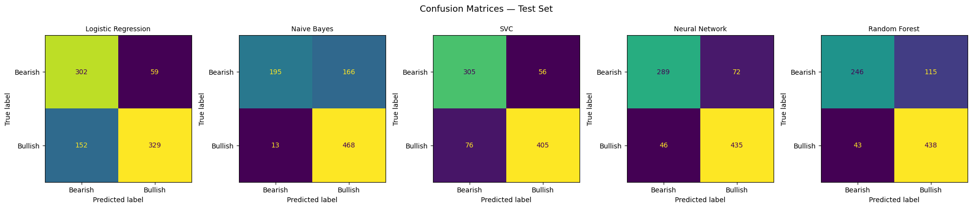
The standout story: Naive Bayes</h3>

<p>Naive Bayes achieved a reasonable overall accuracy of 78.7%, but its confusion matrix reveals a serious flaw. it classified <strong>97.3% of Bullish tweets correctly</strong> while getting <strong>only 54% of Bearish tweets right</strong>. In practice, this model has a strong bias toward predicting Bullish, which would be dangerous in any real application. Missing a bearish signal in a portfolio context is exactly the kind of error that costs money.</p>

<h3 id="logistic-regression-balanced-but-limited">Logistic Regression: balanced but limited</h3>

<p>Logistic Regression was the most balanced model: 84% recall on Bearish tweets and 68% on Bullish. It was also the most interpretable: by examining the model’s coefficients, we can see directly which words drove each prediction.</p>

<p><strong>Top words driving Bullish predictions:</strong> <em>up, beat, raise, rise, higher, buy, upgrade, gain, jump</em></p>

<p><strong>Top words driving Bearish predictions:</strong> <em>down, miss, lower, downgrade, cut, fall, warn, slide, drop, loss</em></p>

<p>These align precisely with how a finance professional would intuitively read a headline. The model has, in effect, learned a basic financial vocabulary from the data alone.</p>

<h3 id="the-neural-network-leads-the-tf-idf-pack">The Neural Network leads the TF-IDF pack</h3>

<p>The Neural Network (a small two-layer architecture) achieved the best balance of accuracy and class recall among the traditional models — 86.3% overall, with 80% recall on Bearish and 91% on Bullish. It also generalised well, suggesting the architecture was not simply memorising the training data.</p>

<hr />

<h2 id="where-the-models-struggled-error-analysis">Where the Models Struggled: Error Analysis</h2>

<p>Examining the Neural Network’s 115 misclassified tweets reveals why this problem is genuinely hard, even for humans.</p>

<p><strong>Predicted Bullish, actually Bearish:</strong></p>
<blockquote>
  <p><em>“More stockmarket volatility, less buying the dip, and slower earnings per share growth ahead, Goldman Sachs says”</em></p>
</blockquote>

<blockquote>
  <p><em>“EIA forecasts U.S. shale oil output to climb by 49,000 barrels a day in December”</em></p>
</blockquote>

<p>The first contains words like “buying” that typically signal Bullish sentiment. The second includes “climb”, a positive word, despite describing an output increase that could be bearish for prices. Context and domain knowledge matter enormously here.</p>

<p><strong>Predicted Bearish, actually Bullish:</strong></p>
<blockquote>
  <p><em>“Fed’s ‘bazooka’ soothes dollar funding squeeze”</em></p>
</blockquote>

<blockquote>
  <p><em>“Jobless Americans to see extra payments as soon as this week”</em></p>
</blockquote>

<p>“Squeeze” and “Jobless” look negative in isolation, but both tweets carry a broadly positive market implication. A word-counting model has no way of knowing this.</p>

<hr />

<h2 id="finbert-context-changes-everything">FinBERT: Context Changes Everything</h2>

<p>FinBERT is a version of BERT, one of the most significant advances in natural language AI, fine-tuned specifically on financial documents. Rather than treating words as isolated signals, it reads each tweet as a sequence and understands relationships between words.</p>

<p>The approach here was to use FinBERT purely as a <strong>feature extractor</strong>: each tweet was passed through the model to produce a rich numerical representation capturing its financial meaning, then a simple Logistic Regression was trained on those representations.</p>

<p>The result: <strong>87.7% accuracy and 0.943 ROC-AUC</strong>, the best of all models tested, with strong recall on both Bearish (87.3%) and Bullish (87.9%) classes.</p>

<p>Crucially, FinBERT is the only model that could plausibly handle tweets like the “bazooka” example above; because it was trained on enough financial text to understand that a central bank intervention, however colourfully described, is typically market-positive.</p>

<hr />

<h2 id="key-takeaways">Key Takeaways</h2>

<p><strong>1. Word-counting methods work, but have clear limits.</strong>
TF-IDF models learned a credible financial vocabulary and performed well on straightforward tweets. They struggle the moment sentiment depends on context rather than individual words.</p>

<p><strong>2. High accuracy can hide dangerous blind spots.</strong>
Naive Bayes looked reasonable on paper but was nearly blind to Bearish signals. In any real-world application like risk management, trade signal generation, news monitoring, recall on each class matters as much as overall accuracy.</p>

<p><strong>3. Financial language is genuinely ambiguous.</strong>
Many misclassified tweets were ambiguous even by human standards. Words like “climb”, “squeeze”, and “bazooka” carry very different meanings depending on what surrounds them. This is precisely the problem FinBERT was built to address.</p>

<p><strong>4. Pre-trained financial models meaningfully outperform bag-of-words.</strong>
FinBERT’s improvement over the best TF-IDF model was modest in percentage terms but consistent across both classes and the gap would likely widen on more complex or nuanced financial text.</p>

<hr />

<p><em>Built using Python, scikit-learn, and HuggingFace Transformers. Dataset: Twitter Financial News Sentiment (Zeroshot / HuggingFace).</em></p>]]></content><author><name>Abdul Malik</name><email>abdul.malik.work@gmail.com</email></author><category term="Projects" /><category term="Python" /><category term="NLP" /><category term="Machine Learning" /><category term="FinBERT" /><category term="Sentiment Analysis" /><category term="Finance" /><summary type="html"><![CDATA[Financial markets move on information, and increasingly, that information flows through social media before it reaches anywhere else. A tweet from an analyst, a headline reposted by a trader, a single word like “downgrade” are all signals that can move prices. The question this project explores is simple: Can a machine be trained to reliably tell a bullish post from a bearish one?]]></summary><media:thumbnail xmlns:media="http://search.yahoo.com/mrss/" url="https://finance.abdulmalik.de/assets/images/twitter_banner.png" /><media:content medium="image" url="https://finance.abdulmalik.de/assets/images/twitter_banner.png" xmlns:media="http://search.yahoo.com/mrss/" /></entry><entry><title type="html">MoneyWise: Gamified Financial Literacy</title><link href="https://finance.abdulmalik.de/2026/03/12/moneywise-credit-game/" rel="alternate" type="text/html" title="MoneyWise: Gamified Financial Literacy" /><published>2026-03-12T00:00:00+01:00</published><updated>2026-03-12T00:00:00+01:00</updated><id>https://finance.abdulmalik.de/2026/03/12/moneywise-credit-game</id><content type="html" xml:base="https://finance.abdulmalik.de/2026/03/12/moneywise-credit-game/"><![CDATA[<h2 id="overview">Overview</h2>

<p>MoneyWise is an interactive browser game built to make financial literacy accessible and engaging. Players navigate a series of real-life financial scenarios like managing credit, spending decisions, and savings while tracking their <strong>Credit Power</strong> and <strong>Savings</strong> in real time.</p>

<p>The core idea: learning personal finance should feel like playing a game, not reading a textbook.</p>

<p><a href="https://moneywisedemo.netlify.app/">Play a live Demo →</a></p>

<h2 id="motivation">Motivation</h2>

<p>Financial literacy is one of the most underdeveloped life skills for young adults. Most people learn about credit scores, interest rates, and budgeting only after making costly mistakes. MoneyWise flips that. It put players in scenarios where the consequences of poor financial decisions are felt in a safe, simulated environment.</p>

<p>The game format naturally drives engagement: every choice has a visible impact on your Credit Power score and Savings balance, creating an immediate feedback loop that textbooks simply can’t replicate.</p>

<h2 id="technical-stack">Technical Stack</h2>

<table>
  <thead>
    <tr>
      <th>Layer</th>
      <th>Technology</th>
    </tr>
  </thead>
  <tbody>
    <tr>
      <td>UI Framework</td>
      <td>React</td>
    </tr>
    <tr>
      <td>Routing</td>
      <td>React Router v6</td>
    </tr>
    <tr>
      <td>State Management</td>
      <td>MobX</td>
    </tr>
    <tr>
      <td>Animations</td>
      <td>CSS Transitions</td>
    </tr>
    <tr>
      <td>Analytics</td>
      <td>Google Analytics</td>
    </tr>
    <tr>
      <td>Deployment</td>
      <td>Netlify</td>
    </tr>
  </tbody>
</table>

<h2 id="core-features">Core Features</h2>

<ul>
  <li><strong>Credit Power tracking</strong> — every decision affects your score, just like real life</li>
  <li><strong>Savings management</strong> — balance short-term spending against long-term goals</li>
  <li><strong>Sequential scenario gameplay</strong> — progress through increasingly complex financial situations</li>
  <li><strong>Interactive decision trees</strong> — multiple-choice paths with distinct financial outcomes</li>
  <li><strong>Progress tracking</strong> — visual feedback on how each choice moves your financial health</li>
</ul>

<h2 id="gameplay-loop">Gameplay Loop</h2>

<ol>
  <li>Player is presented with a real-life financial scenario (e.g. <em>“You need a new phone:  buy outright, finance it, or wait?”</em>)</li>
  <li>Choose from 2–3 options, each with different financial implications</li>
  <li>Credit Power and Savings update immediately based on the choice</li>
  <li>A brief explanation shows why the outcome occurred</li>
  <li>Move to the next scenario</li>
</ol>

<p>This loop reinforces cause-and-effect thinking around financial decisions in a way that sticks.</p>

<h2 id="key-takeaways">Key Takeaways</h2>

<ul>
  <li>Gamification is a genuinely effective delivery mechanism for financial education as engagement stays high when stakes feel real. The duolingo playbook.</li>
  <li>MobX’s observable state makes it easy to keep UI perfectly in sync with game state without boilerplate.</li>
  <li>Designing scenarios requires as much domain knowledge (personal finance) as technical skill. The game is only as good as the quality of its dilemmas.</li>
</ul>

<h2 id="links">Links</h2>

<p>Full source on <a href="https://github.com/leo-lightfoot/FinLearningGamified">GitHub</a> · Live demo at <a href="https://moneywisedemo.netlify.app/">moneywisedemo.netlify.app</a></p>]]></content><author><name>Abdul Malik</name><email>abdul.malik.work@gmail.com</email></author><category term="Projects" /><category term="React" /><category term="MobX" /><category term="JavaScript" /><category term="Financial Literacy" /><category term="Game Design" /><summary type="html"><![CDATA[Overview]]></summary><media:thumbnail xmlns:media="http://search.yahoo.com/mrss/" url="https://finance.abdulmalik.de/assets/images/Fin_Literacy.png" /><media:content medium="image" url="https://finance.abdulmalik.de/assets/images/Fin_Literacy.png" xmlns:media="http://search.yahoo.com/mrss/" /></entry><entry><title type="html">Yield Curve PCA &amp;amp; P&amp;amp;L Attribution</title><link href="https://finance.abdulmalik.de/2026/03/11/yield-curve-pca/" rel="alternate" type="text/html" title="Yield Curve PCA &amp;amp; P&amp;amp;L Attribution" /><published>2026-03-11T00:00:00+01:00</published><updated>2026-03-11T00:00:00+01:00</updated><id>https://finance.abdulmalik.de/2026/03/11/yield-curve-pca</id><content type="html" xml:base="https://finance.abdulmalik.de/2026/03/11/yield-curve-pca/"><![CDATA[<h2 id="overview">Overview</h2>

<p>This project decomposes US Treasury yield curve movements into their principal components, calibrates historical shocks, prices a fixed income portfolio, and attributes P&amp;L under each scenario using FRED data.</p>

<p>The three dominant PCA factors — <strong>level</strong>, <strong>slope</strong>, and <strong>curvature</strong> — explain over 95% of historical yield curve variance, making them powerful tools for scenario analysis and risk attribution.</p>

<h2 id="motivation">Motivation</h2>

<p>Fixed income portfolio managers constantly face the question: <em>why did my portfolio P&amp;L change today?</em> Breaking down P&amp;L into interpretable factors (parallel shift, steepening/flattening, twist) is far more useful than a single unexplained number.</p>

<h2 id="methodology">Methodology</h2>

<h3 id="1-data-collection">1. Data Collection</h3>

<p>Historical US Treasury yields pulled from FRED for maturities: 3M, 6M, 1Y, 2Y, 3Y, 5Y, 7Y, 10Y, 20Y, 30Y.</p>

<h3 id="2-pca-decomposition">2. PCA Decomposition</h3>

<div class="language-python highlighter-rouge"><div class="highlight"><pre class="highlight"><code><span class="kn">from</span> <span class="n">sklearn.decomposition</span> <span class="kn">import</span> <span class="n">PCA</span>
<span class="kn">import</span> <span class="n">pandas</span> <span class="k">as</span> <span class="n">pd</span>
<span class="kn">import</span> <span class="n">numpy</span> <span class="k">as</span> <span class="n">np</span>

<span class="c1"># Compute daily yield changes
</span><span class="n">yield_changes</span> <span class="o">=</span> <span class="n">yields</span><span class="p">.</span><span class="nf">diff</span><span class="p">().</span><span class="nf">dropna</span><span class="p">()</span>

<span class="c1"># Fit PCA
</span><span class="n">pca</span> <span class="o">=</span> <span class="nc">PCA</span><span class="p">(</span><span class="n">n_components</span><span class="o">=</span><span class="mi">3</span><span class="p">)</span>
<span class="n">pca</span><span class="p">.</span><span class="nf">fit</span><span class="p">(</span><span class="n">yield_changes</span><span class="p">)</span>

<span class="c1"># Explained variance
</span><span class="nf">print</span><span class="p">(</span><span class="sa">f</span><span class="sh">"</span><span class="s">PC1 (Level): </span><span class="si">{</span><span class="n">pca</span><span class="p">.</span><span class="n">explained_variance_ratio_</span><span class="p">[</span><span class="mi">0</span><span class="p">]</span><span class="si">:</span><span class="p">.</span><span class="mi">1</span><span class="o">%</span><span class="si">}</span><span class="sh">"</span><span class="p">)</span>
<span class="nf">print</span><span class="p">(</span><span class="sa">f</span><span class="sh">"</span><span class="s">PC2 (Slope): </span><span class="si">{</span><span class="n">pca</span><span class="p">.</span><span class="n">explained_variance_ratio_</span><span class="p">[</span><span class="mi">1</span><span class="p">]</span><span class="si">:</span><span class="p">.</span><span class="mi">1</span><span class="o">%</span><span class="si">}</span><span class="sh">"</span><span class="p">)</span>
<span class="nf">print</span><span class="p">(</span><span class="sa">f</span><span class="sh">"</span><span class="s">PC3 (Curvature): </span><span class="si">{</span><span class="n">pca</span><span class="p">.</span><span class="n">explained_variance_ratio_</span><span class="p">[</span><span class="mi">2</span><span class="p">]</span><span class="si">:</span><span class="p">.</span><span class="mi">1</span><span class="o">%</span><span class="si">}</span><span class="sh">"</span><span class="p">)</span>
</code></pre></div></div>

<h3 id="3-portfolio-pricing">3. Portfolio Pricing</h3>

<p>Each bond in the portfolio is priced under each PCA shock scenario using modified duration and convexity adjustments.</p>

<h3 id="4-pl-attribution">4. P&amp;L Attribution</h3>

<p>Total P&amp;L is decomposed as:</p>

<blockquote>
  <p>ΔP&amp;L = β₁·PC1_shock + β₂·PC2_shock + β₃·PC3_shock + residual</p>
</blockquote>

<h2 id="results">Results</h2>

<table>
  <thead>
    <tr>
      <th>Factor</th>
      <th>Explained Variance</th>
      <th>P&amp;L Contribution</th>
    </tr>
  </thead>
  <tbody>
    <tr>
      <td>Level (PC1)</td>
      <td>82.3%</td>
      <td>-€45,200</td>
    </tr>
    <tr>
      <td>Slope (PC2)</td>
      <td>11.1%</td>
      <td>+€12,800</td>
    </tr>
    <tr>
      <td>Curvature (PC3)</td>
      <td>4.2%</td>
      <td>-€3,100</td>
    </tr>
    <tr>
      <td>Residual</td>
      <td>2.4%</td>
      <td>+€1,500</td>
    </tr>
  </tbody>
</table>

<h2 id="key-takeaways">Key Takeaways</h2>

<ul>
  <li>The level factor dominates — a 25bps parallel shift accounts for the majority of P&amp;L swings</li>
  <li>Slope risk (steepening/flattening) is the second most important driver</li>
  <li>Curvature effects are small but material for barbell/butterfly strategies</li>
</ul>

<h2 id="code--repo">Code &amp; Repo</h2>

<p>Full implementation available on <a href="https://github.com/leo-lightfoot/Yield_Curve_PCA">GitHub</a> and on display at <a href="https://leo-lightfoot.github.io/Yield_Curve_PCA">WebSite</a>.</p>]]></content><author><name>Abdul Malik</name><email>abdul.malik.work@gmail.com</email></author><category term="Projects" /><category term="Python" /><category term="PCA" /><category term="Fixed Income" /><category term="Yield Curve" /><category term="Risk Analytics" /><summary type="html"><![CDATA[Overview]]></summary><media:thumbnail xmlns:media="http://search.yahoo.com/mrss/" url="https://finance.abdulmalik.de/assets/images/Yield_curve.png" /><media:content medium="image" url="https://finance.abdulmalik.de/assets/images/Yield_curve.png" xmlns:media="http://search.yahoo.com/mrss/" /></entry></feed>